We want to drive home the point that along with Neural Network acceleration, we also accelerate data parallelism for classical algorithms, as well. We selected the Fourier Transform because of its historical and continued importance across many industries. As well as the elegance with which is maps to our architecture.
Next up in our algorithm stories series, we want to walk you through how more general-purpose, highly parallelizable algorithms map to our architecture. In this installment, we will talk about one of the most important algorithms of all time, the Fourier transform. An algorithm with its origins in the early 19th century to describe heat propagation in solid bodies, its applications are wide-ranging.
Let’s focus on the implementation and acceleration of the FFT using our Source Mode. If you want to learn more about the FFT itself and its applications, I’ve included a list of my favorite resources below. My personal favorite is the “Three Blue One Brown” video on the Fourier transform.
https://en.wikipedia.org/wiki/Fourier_transform
https://en.wikipedia.org/wiki/Fourier_analysis
If you take away only one thing about the universal application of the FFT, look no further than in your pocket. Modern radio communications rely heavily on frequency domain representation of real-world sampled data. And the way that we get a frequency domain representation of that data is by using the FFT.
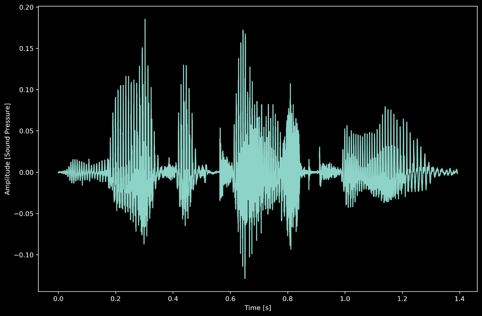
With that motivation, let’s get started with a simple example. Consider the time-domain representation of my voice:
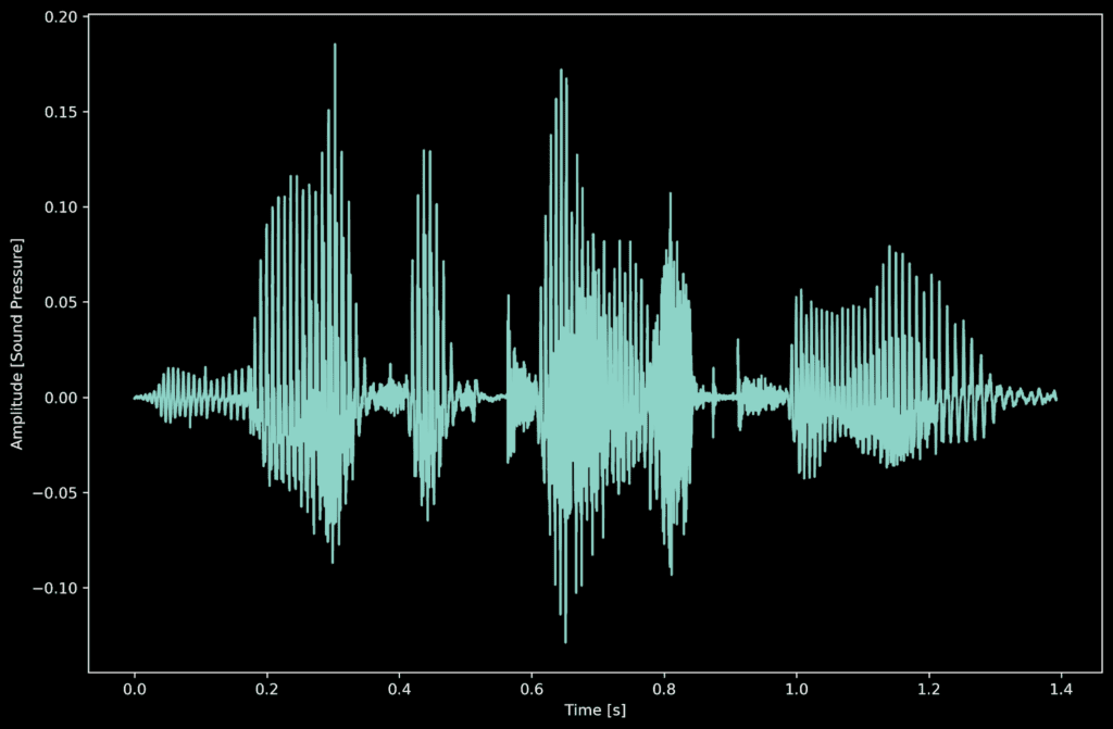
This is a voice recording of me saying, “ the FFT is cool.” You can see it takes me about 1.5 seconds to say that. But what is the average frequency composition of voice for these 1.5 seconds? Using the FFT, we can generate a frequency domain representation. Here we plot the amplitude of a signal versus its frequency composition.
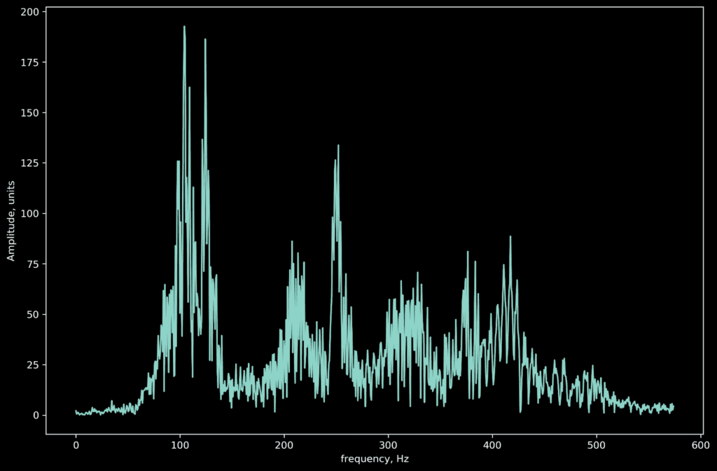
According to Wikipedia: the human male voice can produce frequencies from 85 to 180 Hz. So it looks like it checks out!
To generate the FFT, we will look at the Cooley Tukey algorithm developed in the mid 20th century. This algorithm completes the FFT in O(n*log(n)) and is well suited to map the quadric processor architecture.
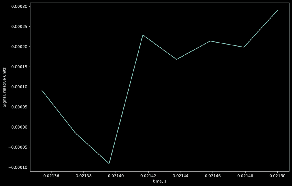
For illustration purposes, we can take a sample or “window” from my audio recording consisting of 8 points. By taking an 8 sample window, we will effectively be performing an “8-Point FFT.” For ease of explanation and the sake of illustration, we will map the FFT on a 2x2 architecture instance. That’s a vector that has shape 8x1:
A = [-0.00064087 -0.00062561 -0.00074768 -0.00068665 -0.00065613 -0.00054932 -0.0005188 -0.00061035]
To implement the FFT algorithm, we will following these steps:
We can remap the data inside of our array using index manipulation. Reversing the index arrives at the desired remapping. Have a look at the effect on an 8 point FFT. The same will be valid for any arbitrary power of 2 - point implementation.
The code for such remapping looks something like this:
  template
  INLINE void fetchInputIndexBitReversed(OcmInOutSignalTensorShape ocmIn,
                                         qVar_t          qInput[],
                                         std::int32_t              signalRowOffset = 0,
                                         std::int32_t              signalChOffset  = 0) {
    constexpr std::int32_t numTilesPerInputPoints =
      roundUpToNearestMultiple(inputPoints, Epu::numArrayCores) / Epu::numArrayCores;
    Rau::config(ocmIn);
    qVar_t  qLocalCoreIndx = qRow<> * Epu::coreDim + qCol<>;
    constexpr std::int32_t complexCount   = 2;  // real and imaginary
    for(std::uint32_t chIndx = 0; chIndx < complexCount; chIndx++) {
      for(std::uint32_t tileIndx = 0; tileIndx < numTilesPerInputPoints; tileIndx++) {
        qVar_t coreIndx  = tileIndx * Epu::numArrayCores + qLocalCoreIndx;
        qVar_t rCoreIndx = bitReversal(coreIndx);
        std::int32_t          arrayIndx = chIndx * numTilesPerInputPoints + tileIndx;
        qInput[arrayIndx] = Rau::Load::oneTile(0, signalChOffset + chIndx, signalRowOffset, rCoreIndx, ocmIn);
        if(coreIndx >= inputPoints) {
          qInput[arrayIndx] = 0;
        }
      }
    }
  }
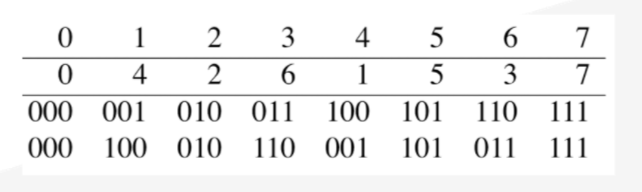
The above data remapping leads to a rearrangement of the vector in the following fashion:
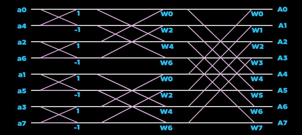
The rearranged input vector is on the left. And the output vector is shown on the right after the Cooley-Tukey algorithm is applied.
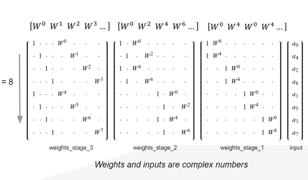
If you were to implement the algorithm as matrix multiplication, with 3 matrix products of sparse representations. You would think this would lead to poor spatial array utilization. However, we can pack the products and share data cleverly to execute the algorithm efficiently.
Let’s simplify our representation of the quadric architecture into 4 simple rectangles. Each representing a Vortex Core. Any variable depicted within the rectangle is stored locally within that Vortex Core’s local memory.
Using the periphery load-store units. We write the remapped vector linearly L-R, T-B into the core. When we’ve reached the end, we return to the upper left Vortex Core and then write the L-R, T-B. In our simple case of an 8-point FFT mapping to a 4 core architecture instance, this results in the following data layout:
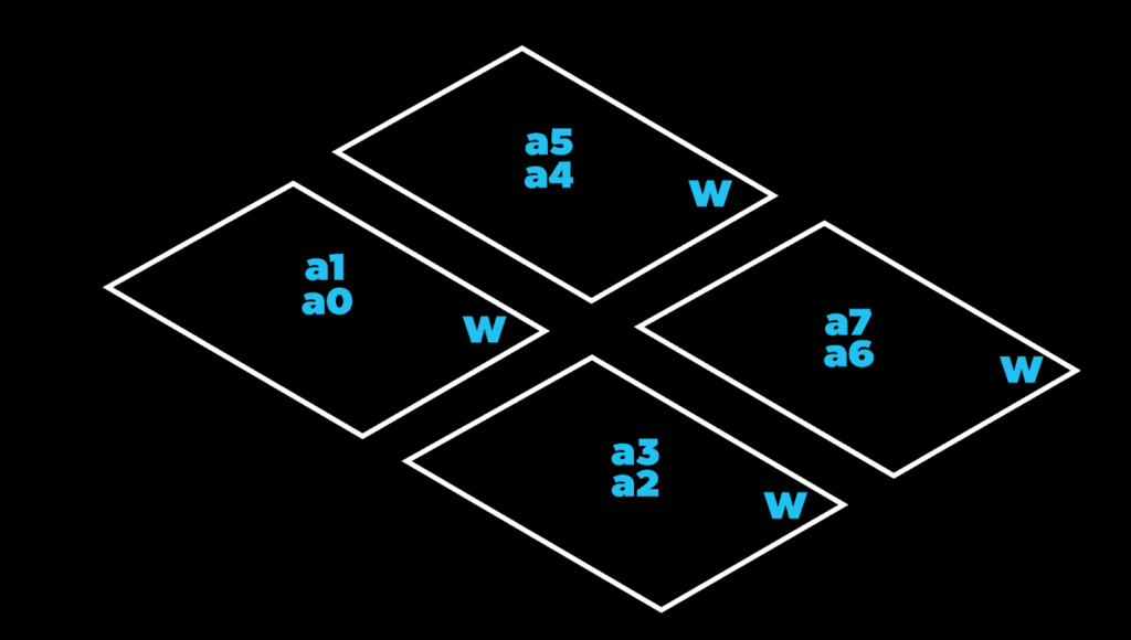
Now we can execute the stage 1 product using neighboring data. If we look at the top row, we need to complete the product a0 + W0*a4 and a1 + W0*a5. The inputs a0 and a1 are stored locally. While the inputs a4 and a5 are stored in our nearest neighbors. The opposite is true for the core the east of it (upper right core). Using single cycle neighbor access, we can publish our data to our neighboring Vortex Cores and consume them in our own product. You can think of the first stage mapping of the 8-point 1D FFT as mapping to row-wise data sharing.
Now we can execute the stage 2 products using neighboring data. If we look at the top row again, we need to perform the products of the subsequent stage with information now stored in our North-South neighbors. So we can publish the intermediate values north and south to be used in that computation. You can think of the second stage mapping of the 8-point 1D FFT as mapping to column-wise data sharing.
For the third and final stage, notice that the required data has been folded inside each Vortex Core. The information is stored locally inside of the register file of the Vortex Core that needs it. So to complete the final products, we can simply fetch the intermediate products stored locally to finish out the FFT. You can think of the third stage mapping of the 8-point 1D FFT as mapping to depth-wise or channel-wise data sharing.
The 8-point FFT is now completed. The upper left core stores the A0 and A1, the upper right Vortex Core containing A4 and A5, the lower-left Vortex Core containing A2 and A3, and the final core containing A6 and A7. We chose this combination of array size and FFT-point window because it covers all cases that arise in other varieties. No matter what, there will be some combination of row-wise, column-wise, and channel-wise data sharing.
Here is a short animation of the above description!
We have generalized the concept for all N-point variants based upon the dimensionality of the core array. Of course, running an N-point FFT on the q16 processor would be easy. However, the q16 will process a 512 point FFT similarly to the example we walked through today. Instead of 3 stages, it would require 9. As a part of the quadric SDK, we provide FFT library calls that handle the data manipulation. Here is a snippet of the relevant source for determining the layout. We present this as an example to give you an idea of the power and compatibility of our high-performance data-parallel processing architecture. For more information about the 1D FFT library function, check out our documentation :
© Copyright 2024 Quadric All Rights Reserved Privacy Policy